The unit assessment for the Waves & Radiation unit of National 5 is scheduled for next week. These notes will be useful as you prepare for the test.
Thanks to Mr Noble for sharing these notes.
with mr mackenzie

podcasts go in this category for the feed to iTunes
The unit assessment for the Waves & Radiation unit of National 5 is scheduled for next week. These notes will be useful as you prepare for the test.
Thanks to Mr Noble for sharing these notes.
Last week, we learned about internal resistance of cells. Page 24 of your printed notes explains how to use a simple series circuit containing a cell, resistance box, ammeter and voltmeter to determine the internal resistance of the cell. By plotting a graph of your dat, with current on the x-axis and voltage on the y-axis, you can find the internal resistance of the cell.
The video below shows the same type of experiment, but uses a potato and two different metals in place of a normal cell. Watch the video and note the values of I and V each time the resistance is changed – remember to pause the video each time so you can write the results. Just scroll back if you miss any.
Now plot a graph with current along the x-axis and TPD along the y-axis. If you don’t have any sheets of graph paper handy, there is a sheet available to download using the button at the end of this post. Alternatively, print a sheet from a graph paper site or use google sheetsto plot your results.
Draw a best-fit straight line for the points on your graph and find the gradient of the line. When calculating gradient, remember to convert the current units from microamps (uA) to amps (A).
The gradient of your straight line will be a negative number. The gradient is equal to -r, where r is the internal resistance of the potato cell used in the video.
You can obtain other important information from this graph;
X-rays are a form of electromagnetic radiation. They have a much higher frequency than visible light or ultraviolet. The diagram below, taken from Wikipedia, shows where x-rays sit in the electromagnetic spectrum.

Wilhelm Röntgen discovered x-rays and the image below is the first x-ray image ever taken. It shows Mrs. Röntgen’s hand and wedding ring. The x-ray source used by Röntgen was quite weak, so his wife had to hold her hand still for about 15 minutes to expose the film. Can you imagine waiting that long nowadays?

This was the first time anyone had seen inside a human body without cutting it open. Poor Mrs. Röntgen was so alarmed by the sight of the image made by her husband that she cried out “I have seen my death!” Or, since she was in Germany, it might have been
“Ich habe meinen Tod gesehen!“
that she actually said.
Röntgen continued to work on x-rays until he was able to produce better images. The x-ray below was taken about a year after the first x-ray and you can see the improvements in quality.

Notice that these early x-rays are the opposite of what we would expect to see today. They show dark bones on a lighter background while we are used to seeing white bones on a dark background, such as the x-ray shown below. The difference is due to the processing the film has received after being exposed to x-rays.
 In hospitals, x-rays expose a film which is then developed and viewed with bright light. X-rays are able to travel through soft body tissue and the film behind receives a large exposure. The x-rays darken the film. More dense structures such as bone, metal fillings in teeth, artificial hip/knee joints, etc. block the path of x-rays and prevent them from reaching the film. Unexposed regions of the film remain light in colour.
Röntgen’s x-ray films would have involved additional processing steps. The exposed films were developed and used to create a positive. In creating a positive, light areas become dark and dark areas become light. So the light and dark areas in Röntgen’s x-rays are the opposite of what we see today. Our modern method makes it easier to detect issues in the bones as they are the lighter areas.
Röntgen was awarded the first ever Nobel Prize for Physics in 1901 for his pioneering work in this field of physics.
I have attached a recording of a short BBC radio programme about the first x-ray and what people in the Victorian era thought of these new images. Click on the player at the end of this post or listen to it in iTunes.
This document will help you to generate ideas for your assignment.
Here is the document you will need for the earthquakes assignment. We have equipment for you to carry out practical activities 2 and 3. You will also need the Audacity guide.
We’re going to start the researching physics unit and assignment next week. Before we go to the computer room, please watch the attached video so you will have some ideas about the science of earthquakes and how they can be detected.
This is a large video file – make sure you are connected to wifi before downloading.
Please do not stream the video as this will prevent others from viewing at the same time. Download the file before you start to watch.
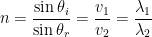
We met refraction during the National 5 course. At Higher level, we are interested in the relationship between the angles of incidence θi and refraction θr.
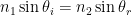
Snell’s law tells us that
Usually material 1 is air, and so 
where n is the absolute refractive index of material 2. Since the refractive index is equal to the ratio of the ray’s speed v in materials 1 & 2 and also equal to the ratio of the wave’s wavelength λ in materials 1 & 2, we can show that
Read more about Snells’s law here.
 and refractive index n are related by

Here are some applications of total internal reflection here. You can test your knowledge of refraction with this interactive simulation.
I have attached a pdf with some notes and questions on refraction, total internal reflection and critical angle.
The second programme is all about the current state of car safety.
We follow a car safety team at Volvo as they prepare to crash two cars together to collect forces data, learn how emergency medicine procedures are changing to improve outcomes for car accident casualties, and learn how sensors are used to monitor the human body’s response to a collision.
Please watch both programmes before Thursday 18th February.
As with the first video, please check you are connected to wifi before downloading as the video file is quite big.
We’re going to start work on the assignment task next week. You’ll spend 2-3 periods researching car safety online and choosing a particular topic to explore in more depth. Before we go into the ICT room, I’d like you to watch two videos about car safety.
The first programme looks back at the history of car accidents and the work that has been done to reduce deaths on the road. While many of the clips shown are quite old, they show just how far we have come in our understanding of the science behind making cars more safe.
Please right click on the link below and save your own copy of the file, rather than streaming it.
Check you’re using wifi before downloading – it’s a big file!
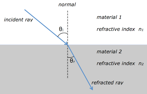
Diffraction is a test for wave behaviour. When a ray of light passes through a diffraction grating, the energy of the incident beam is split into a series of interference fringes. Constructive interference is occurring at each location where a fringe (or spot) is observed because the rays are in phase when they arrive at these points.
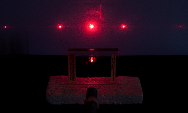
Find out about diffraction gratings here.
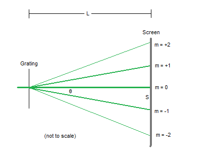
We can measure the relative positions of the fringes in a diffraction pattern to determine the wavelength of the light used. The diffraction grating equation is
where
Here is an infrared diffraction experiment you can try at home to calculate the wavelength of the infrared LED in a remote control.
I’ve attached a set of pdf notes and questions on diffraction. These notes use n rather than m for the diffracted order.