
Higher
capacitors
You recently completed the topic on capacitors in dc circuits, finishing off with a detailed study of the graphs obtained for current & voltage against time when a capacitor is charged or discharged through a series resistor. There are some additional notes and practice questions at the end of this post but please watch the embedded video clips first.
This introduction to capacitors from the nice people at Make Magazine is a good starting point.
The S-cool revision site has some helpful notes and illustrations on capacitor behaviour; try page 1 (how capacitors work) and page 2 (charging and discharging).
There is information on charging and discharging capacitors on BBC Bitesize.
Use your knowledge of capacitor behaviour to explain how a flashing neon bulb can be controlled using a capacitor & resistor arranged in series. Here is a short video introduction to help with that.
Blinking Neon Bulb (5F30.60A) from Ricardo Alarcon on Vimeo.
There are people working to replace heavy battery packs with modern, high capacitance devices called supercapacitors. These supercapacitors have superior energy storage compared to the normal electrolytic capacitors you will have used in class. This video goes one step further and shows the fun you could have with an ultracapacitor. Do not try this at home!
Of course, you can always make your own capacitor with paper and electrically conductive paint.
Finally, you looked at capacitors in ac circuits. You need to know that a capacitor will allow an ac current to flow. The current in such a circuit will increase as the current increases. Mr Mallon’s site has a revision activity about capacitors in ac circuits.
Now download the pdf below. It contains notes to help with your prelim revision and some extra capacitor problems.
Thanks to Fife Science for the original pdf from Martin Cunningham.

E-Book PDF: Open in New Window | Download
internal resistance
Last week, we learned about internal resistance of cells. Page 24 of your printed notes explains how to use a simple series circuit containing a cell, resistance box, ammeter and voltmeter to determine the internal resistance of the cell. By plotting a graph of your dat, with current on the x-axis and voltage on the y-axis, you can find the internal resistance of the cell.
The video below shows the same type of experiment, but uses a potato and two different metals in place of a normal cell. Watch the video and note the values of I and V each time the resistance is changed – remember to pause the video each time so you can write the results. Just scroll back if you miss any.
Now plot a graph with current along the x-axis and TPD along the y-axis. If you don’t have any sheets of graph paper handy, there is a sheet available to download using the button at the end of this post. Alternatively, print a sheet from a graph paper site or use google sheetsto plot your results.
Draw a best-fit straight line for the points on your graph and find the gradient of the line. When calculating gradient, remember to convert the current units from microamps (uA) to amps (A).
The gradient of your straight line will be a negative number. The gradient is equal to -r, where r is the internal resistance of the potato cell used in the video.
You can obtain other important information from this graph;
- Extend your best fit line so that it touches the y-axis. The value of the TPD where the line touches the y-axis is equal to the EMF of the cell. (Explanation: on the y-axis, I is zero so TPD = EMF)
- Now extend the best-fit line so that it touches the x-axis, the current at that point is the short-circuit current – this is the maximum current that the potato cell can provide when the variable resistor is removed from the circuit altogether and replaced with just a wire.
E-Book PDF: Open in New Window | Download
Higher assignment – LEDs and optical fibres
This document will help you to generate ideas for your assignment.
E-Book PDF: Open in New Window | Download
Higher assignment – earthquakes
Here is the document you will need for the earthquakes assignment. We have equipment for you to carry out practical activities 2 and 3. You will also need the Audacity guide.
E-Book PDF: Open in New Window | Download
higher assignment video – earthquakes
We’re going to start the researching physics unit and assignment next week. Before we go to the computer room, please watch the attached video so you will have some ideas about the science of earthquakes and how they can be detected.
This is a large video file – make sure you are connected to wifi before downloading.
Please do not stream the video as this will prevent others from viewing at the same time. Download the file before you start to watch.
Podcast: Play in new window | Download
refraction, critical angle and total internal reflection
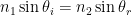
We met refraction during the National 5 course. At Higher level, we are interested in the relationship between the angles of incidence θi and refraction θr.
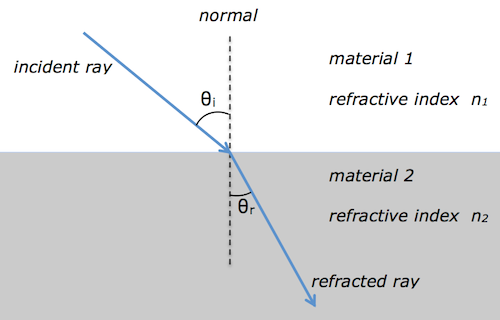
Snell’s law tells us that
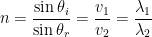
Usually material 1 is air, and so 

where n is the absolute refractive index of material 2. Since the refractive index is equal to the ratio of the ray’s speed v in materials 1 & 2 and also equal to the ratio of the wave’s wavelength λ in materials 1 & 2, we can show that
Read more about Snells’s law here.
total internal reflection
 and refractive index n are related by

Here are some applications of total internal reflection here. You can test your knowledge of refraction with this interactive simulation.
I have attached a pdf with some notes and questions on refraction, total internal reflection and critical angle.
E-Book PDF: Open in New Window | Download
diffraction
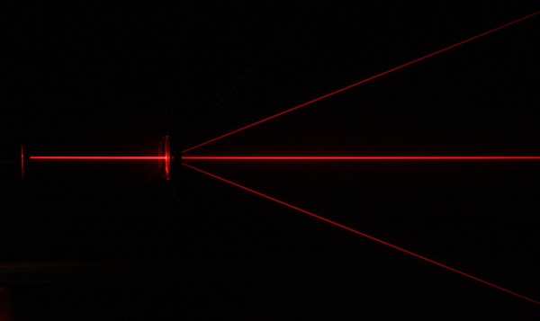
red laser beam passing through a diffraction grating. image: en.academic.ru
Diffraction is a test for wave behaviour. When a ray of light passes through a diffraction grating, the energy of the incident beam is split into a series of interference fringes. Constructive interference is occurring at each location where a fringe (or spot) is observed because the rays are in phase when they arrive at these points.
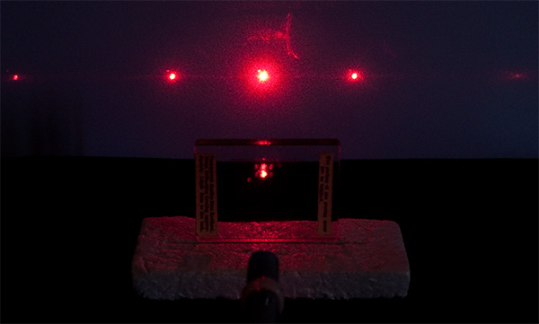
image: microscopy uk
Find out about diffraction gratings here.
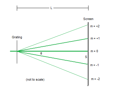
image: laserpointerforums.com
We can measure the relative positions of the fringes in a diffraction pattern to determine the wavelength of the light used. The diffraction grating equation is

where
- m is the diffracted order – some resources may use n instead of m
- λ is the wavelength
- d is the line spacing.
Here is an infrared diffraction experiment you can try at home to calculate the wavelength of the infrared LED in a remote control.
I’ve attached a set of pdf notes and questions on diffraction. These notes use n rather than m for the diffracted order.
E-Book PDF: Open in New Window | Download
the photoelectric effect
We learned about the photoelectric effect this week. This video has a similar demonstration to the gold leaf electroscope experiment I showed you in class and includes an explanation of the process.
Click on the picture below to download the simulation we used to investigate the effect of irradiance on frequency on photocurrent. You’ll be prompted to install Java if you don’t have it already.
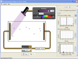
Once the animation is running, you can;
- change the metal under investigation (we used zinc in class)
- vary the wavelength of the incident light
- vary the irradiance of the incident light.
Notice that below the threshold frequency you can’t get any photoelectrons, even if you set the light to its brightest setting.
Compare your results to the graphs provided in your notes.
I have attached some notes & questions on the photoelectric effect. Click on the link below to download a copy.
E-Book PDF: Open in New Window | Download
revision notes for higher ODU resit
I’ve attached a set of notes to help with your revision for the Our Dynamic Universe resit on Tuesday. Remember that the resit paper will have knowledge questions only, so focus on the unit content during your revision rather than practising numerical problems.
Thanks to Mr Noble for sharing his ODU notes.
E-Book PDF: Open in New Window | Download